Table of Contents
Introduction
In dynamic contrast-enhanced (DCE) MRI, pharmacokinetic (PK) modeling can be used to quantify tissue physiology. Parameters describing the tissue microvasculature can be derived by fitting a pharmacokinetic model, e.g. a compartment model, to the dynamic data. This view offers a comprehensive set of tools to perform pharmacokinetic analysis.
Contact information
If you have any questions, need support, find a bug or have a feature request, feel free to contact us at www.mitk.org.
Citation information
If you use the view for your research please cite our work as reference:
Debus C and Floca R, Ingrisch M, Kompan I, Maier-Hein K, Abdollahi A, Nolden M, MITK-ModelFit: generic open-source framework for model fits and their exploration in medical imaging – design, implementation and application on the example of DCE-MRI. https://doi.org/10.1186/s12859-018-2588-1 (BMC Bioinformatics 2019 20:31)
Time series and mask selection
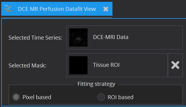
In principle, every model can be fitted on the entire image. However, for model configuration reasons (e.g. AIF required) and computational time cost, this is often not advisable. Therefore, apart from the image to be fitted (Selected Time Series), a ROI segmentation can be defined (Selected Mask), within which model fitting is performed. The view currently offers Pixel based and/or ROI based averaged fits of time-varying curves. The ROI based fitting option becomes enabled, if a mask is selected.
Supported models
Currently the following pharmacokinetic models for gadolinium-based contrast agent are available:
- The descriptive Brix model [1]
- The standard Tofts model [2]
- The extended Tofts model [3]
- The two compartment exchange model (2CXM) [4, 5]
Model settings
Model specific settings
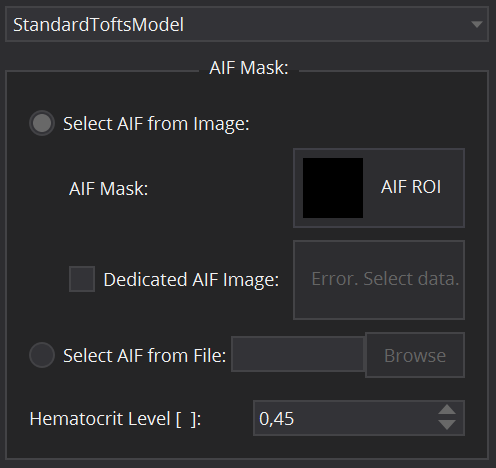
Selecting one of the supported models will open below tabs for further configuration of the model.
- The descriptive Brix model requires only definition of the duration of the bolus, i.e. the overall time of the injection (Injection Time [min]).
- The standard Tofts model, the extended Tofts model and the 2CXM are compartment models that require the input of the concentration time curve in the tissue feeding artery, the arterial input function (AIF).
In the DCE MR Perfusion Datafit View, the arterial input function can be defined in several ways. For patient individual image derived AIFs, select the radio button Select AIF from Image. In that case, a segmentation ROI for the artery has to be selected. This can be done by clicking on the AIF Mask selection widget and selecting a suitable AIF segmentation from the data loaded in the Data Manager. In cases where the respective artery does not lie in the same image as the investigated tissue (e.g. in animal experiments, where a slice through the heart is used for AIF extraction), a dedicated AIF image can be selected using the corresponding Dedicated AIF image selection widget.
An alternative option is to define the AIF via an external file by selecting Select AIF from File (e.g. for population derived AIFs or AIFs from blood sampling). By clicking the Browse button, one can select a csv file that holds the AIF values and corresponding timepoints (in tuple format (Time, Value)).
Caution: the file must not contain a header line, but the first line must start with Time and Intensity values.
Furthermore, the Hematocrit Level has to be set (from 0 to 1) for conversion from whole blood to plasma concentration. It is set as default to the literature value of 0.45.
Signal to concentration conversion settings
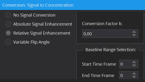
Most models require contrast agent concentration values as input rather than raw signal intensities (i.e. all compartment models). The DCE MR Perfusion DataFit View offers a variety of tools for the conversion from signal to concentration: by means of relative and absolute signal enhancement and via a T1-map calculated by the variable flip angle method. A more detailed description of these conversion methods can be found here: The DCE Concentration Curve Converter View. For the conversion methods, a baseline image prior to contrast agent arrival is required. In many dynamic data sets, multiple images are part of the baseline. The Baseline Range Selection allows for selection of a range of time frames, from which the average image (along the time dimension) is calculated and set as baseline input image. Remark: The number of the first time frame is 0.
Start parameter
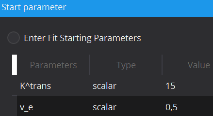
In cases of noisy data it can be useful to define the initial starting values of the parameter estimates, at which optimization starts, in order to prevent optimization results in local optima. Each model has default scalar values (applied to every voxel) for initial values of each parameter, however these can be adjusted. Moreover, initial values can also be defined locally for each individual voxel via starting value images. To load a starting value image, change the Type from scalar to image. This can be done by double-clicking on the type cell. In the Value column, selection of a starting value image will be available.
Constraints settings
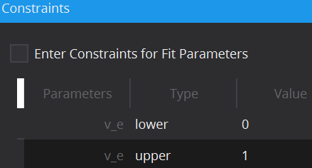
To limit the fitting search space and to exclude unphysical/illogical results for model parameter estimates, constraints to individual parameters as well as combinations can be imposed. Each model has default constraints, however, new ones can be defined or removed by the + and – buttons in the table. The first column specifies the parameter(s) involved in the constraint (if multiple parameters are selected, their sum will be used) by selection in the drop down menu. The second column Type defines whether the constraint defines an upper or lower boundary. Value defines the actual constraint value, that should not be crossed, and Width allows for a certain tolerance width.
Executing a fit
In order to distinguish results from different model fits to the data, a Fitting name can be defined. As default, the name of the model and the fitting strategy (pixel/ROI) are given. This name will then be appended by the respective parameter name.
For development purposes and evaluation of the fits, the option Generate debug parameter images is available. Enabling this option will result in additional parameter maps displaying the status of the optimizer at fit termination. In the following definitions, an evaluation describes the process of cost function calculation and evaluation by the optimizer for a given parameter set.
- Stop condition: Reasons for the fit termination, i.e. criterion reached, maximum number of iterations,...
- Optimization time: The overall time from fitting start to termination.
- Number of iterations: The number of iterations from fitting start to termination.
- Constraint penalty ratio: Ratio between evaluations that were penalized and all evaluations. 0.0 means no evaluation was penalized; 1.0 all evaluations were. Evaluations that hit the failure threshold count as penalized, too.
- Constraint last failed parameter: Ratio between evaluations that were beyond the failure threshold. 0.0 means no evaluation was a failure (but some may be penalized).
- Constraint failure ratio: Index of the first (in terms of index position) parameter, which failed the constraints in the last evaluation.
After all necessary configurations are set, the button Start Modelling is enabled, which starts the fitting routine. Progress can be seen in the message box on the bottom. Resulting parameter maps will afterwards be added to the Data Manager as sub-nodes of the analyzed 4D image.
FAQs
- I generated a parameter map using a pharmacokinetic model (e.g. Standard Tofts model), but I get unreasonable voxel values. What could be the reason for this?
Pharmacokinetic models are fitted to concentration time curves and not signal time curves. Please make sure you have converted the dynamic signal curves to concentration time curves, which you can do in the "DCE MR Perfusion DataFit View" under the tab "Conversion: Signal to Concentration". Another reason might be that the fitting routine got caught up in a local rather than a global minimum and therefore the fitting results are poor parameter estimates. This can be improved by setting reasonable initial parameters and fitting constraints in the "Start parameter" and "Constraints" tabs.
- I have generated a parameter map and it is shown as data node in the data manager. Why can't I see it in the standard display window?
You might be in a slice of a 3D image, in which the map is not visible. Right-click on the parameter map and select "Reinit". Now you can scroll through the slices until you see the map in the standard display.
Make sure that the "Concentration" node is toggled off.
The level-window might be set such that the map is not visible. When the map is open in the standard display, right-click on the slider and select "Use optimized level-window". Afterwards you can fine-tune the level-window by left-click on the slider and moving the mouse up/down or left/right.
Other nodes in the data manager could potentially be displayed if not deselected. To make sure that only the paramenter maps are visible, right click on the parameter map and select "Show only selected nodes".
- Why are my K^trans values much higher than literature values?
In MITK, K^trans values are reported in units of ml/min/100ml (which can be e.g. seen by right clicking on the map, selecting "Show details" and scrolling to the field "modelfit.parameter.unit".). Literature values are sometimes reported in units of min-1, which will be smaller by a factor of 100.
- What are the exact formulas for relative and absolute signal conversion and how should I set the factor k?
You can find a detailed description in the documentation of the concentration curve converter view. Either by opening the view in the workbench and pressing F1 or here: The DCE Concentration Curve Converter View.
The proportionality factor k is dependent on many different factors and is usually not known. However, it does not need to be known as long as k is tissue independent. When fitting an AIF-based pharmacokinetic model based on the standard tracer-kinetic theory of linear and stationary systems, which is e.g. true for the standard Tofts model, k cancels out because it is the same for blood and tissue. Therefore, you can for example just set k = 1.0 (which is also set as default value).
- How can I load the AIF from a file? Which format is needed?
You can load the previously generated AIF as a .csv (or .txt) file. In this file, the AIF values and corresponding timepoints are arranged in the tuple format (timepoint, AIF value), e.g. for the timepoints (0.0, 1.0, 2.0) and AIF values (0.0, 1.5, 5.0) the file would look like this:
0.0, 0.0
1.0, 1.5
2.0, 5.0
Please be aware that the file must not contain a header line, but the first line must already start with timepoints and AIF values.
References/Literature
- [1] Brix G, Semmler W, Port R, Schad LR, Layer G, Lorenz WJ. Pharmacokinetic parameters in CNS Gd-DTPA enhanced MR imaging. J Comput Assist Tomogr. 1991;15:621–8.
- [2] Tofts PS, Kermode AG. Measurement of the blood-brain barrier permeability and leakage space using dynamic MR imaging. 1. Fundamental concepts. Magn Reson Med. 1991;17:357–67.
- [3] Sourbron SP, Buckley DL. On the scope and interpretation of the Tofts models for DCE-MRI. Magn Reson Med. 2011;66:735–45.
- [4] Brix G, Kiessling F, Lucht R, Darai S, Wasser K, Delorme S, et al. Microcirculation and microvasculature in breast tumors: Pharmacokinetic analysis of dynamic MR image series. Magn Reson Med. 2004;52:420–9.
- [5] Sourbron, Buckley. Tracer kinetic modelling in MRI: estimating perfusion and capillary permeability - pdf. Phys Med Biol. 2012. https://iopscience.iop.org/article/10.1088/0031-9155/57/2/R1/pdf. Accessed 1 May 2016.
