This view provides the user interface for Fiberfox [1,2,3], an interactive simulation tool for defining artificial white matter fibers and generating corresponding diffusion-weighted images. Arbitrary fiber configurations like bent, crossing, kissing, twisting, and fanning bundles can be intuitively defined by positioning only a few 3D waypoints to trigger the automated generation of synthetic fibers. From these fibers a diffusion-weighted signal is simulated using a flexible combination of various diffusion models. Instead of using manually created artificial fiber bundles, fibers obtained in any other way, e.g. using fiber tractography, can be used to simulate the signal (Example: ISMRM Tractography Challenge). The simulation can be modified using specified acquisition settings such as gradient direction, b-value, image size, image resolution, echo time, and much more. Additionally it enables the simulation of magnetic resonance artifacts including thermal noise, Gibbs ringing, N/2 ghosting, aliasing, susceptibility distortions, eddy currents and motion artifacts. The employed parameters can be saved and loaded as xml file with the ending ".ffp" (Fiberfox parameters). It is furthermore possible to add artifacts to an already existing diffusion-weighted image.

Available sections:

Fiber Definition
Signal Generation
Known Issues
References

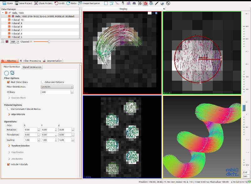
Fig. 1: Screenshot of the Fiberfox framework. The four render windows display an axial (top left), sagittal (top right) and coronal (bottom left) 2D cut as well as a 3D view of a synthetic fiber helix and the fiducials used to define its shape. In the 2D views the helix is superimposing the baseline volume of the corresponding diffusion-weighted image. The sagittal render window shows a close-up view on one of the circular fiducials.

Fiber Definition

Fiber strands are defined simply by placing markers in a 3D image volume. The fibers are then interpolated between these fiducials.

Example:

Chose an image volume to place the markers used to define the fiber pathway. If you don't have such an image available switch to the "Signal Generation" tab, define the size and spacing of the desired image and click "Generate Image". If no fiber bundle is selected, this will generate a dummy image that can be used to place the fiducials.
Start placing fiducials at the desired positions to define the fiber pathway. To do that, click on the button with the circle pictogram, then click at the desired position and plane in the image volume and drag your mouse while keeping the button pressed to generate a circular shape. Adjust the shape using the control points (Fig. 2). The position of control point D introduces a twist of the fibers between two successive fiducials. The actual fiber generation is triggered automatically as soon as you place the second control point.
In some cases the fibers are entangled in a way that can't be resolved by introducing an additional fiber twist. Fiberfox tries to avoid these situations, which arise from different normal orientations of succeeding fiducials, automatically. In rare cases this is not successful. Use the double-arrow button to flip the fiber positions of the selected fiducial in one dimension. Either the problem is resolved now or you can resolve it manually by adjusting the twist-control point.
To create non elliptical fiber profile shapes switch to the Fiber Extraction View. This view provides tools to extract subesets of fibers from fiber bundles and enables to cut out arbitrary polygonal fiber shapes from existing bundles.

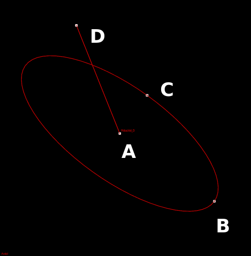
Fig. 2: Control points defining the actual shape of the fiducial. A specifies the fiducials position in space, B and C the two ellipse radii and D the twisting angle between two successive fiducials.

Fiber Options:

Real Time Fibers: If checked, each parameter adjustment (fiducial position, number of fibers, ...) will be directly applied to the selected fiber bundle. If unchecked, the fibers will only be generated if the corresponding button "Generate Fibers" is clicked.
Fiber Distribution: Specifies if the fiber distribution inside the bundle follows a uniform or normal distribution.
# Fibers: Specifies the number of fibers that will be generated for the selected bundle.
Advanced Options: Show/hide advanced options
Fiber Sampling: Adjusts the distenace of the fiber sampling points (in mm). A higher sampling rate is needed if high curvatures are modeled.
Tension, Continuity, Bias: Parameters controlling the shape of the splines interpolation the fiducials. See Wikipedia for details.

Fiducial Options:

Use Constant Fiducial Radius: If checked, all fiducials are treated as circles with the same radius. The first fiducial of the bundle defines the radius of all other fiducials.
Align with grid: Click to shift the selected fiducial center points to the next voxel center.

Operations:

Rotation: Define the rotation of the selected fiber bundle around each axis (in degree).
Translation: Define the translation of the selected fiber bundle along each axis (in mm).
Scaling: Define a scaling factor for the selected fiber bundle in each dimension.
Transform Selection: Apply specified rotation, translation and scaling to the selected Bundle/Fiducial
Copy Bundles: Add copies of the selected fiber bundles to the datamanager.
Join Bundles: Add new bundle to the datamanager that contains all fibers from the selected bundles.
Include Fiducials: If checked, the specified transformation is also applied to the fiducials belonging to the selected fiber bundle and the fiducials are also copied.

Signal Generation

To generate an artificial signal from the input fibers we follow the concepts recently presented by Panagiotaki et al. in a review and taxonomy of different compartment models: a flexible model combining multiple compartments is used to simulate the anisotropic diffusion inside (intra-axonal compartment) and between axons (inter-axonal compartment), isotropic diffusion outside of the axons (extra-axonal compartment 1) and the restricted diffusion in other cell types (extra-axonal compartment 2) weighted according to their respective volume fraction.

A diffusion-weighted image is generated from the fibers by selecting the according fiber bundle in the "Fiber Bundle" combobox and clicking "Generate Image". If some other diffusion-weighted image is selected together with the fiber bundle, Fiberfox directly uses the parameters of the selected image (size, spacing, gradient directions, b-values) for the signal generation process. Additionally a binary image can be selected that defines the tissue area. Voxels outside of this mask will contain no signal, only noise and other effects induced by the acquisiton (ghosts etc.). If a save path is specified, the simualted image will be saved at this location. Eventually generated log files (e.g. recording the head motion) are also saved at this location. If not path is specified, the simualted image will only appear in the data manager and has to be saved manually. Logfiles are then saved in the system specific temp directory.

If no fiber bundle but a diffusion-weighted image is selected, the specified artifacts are added to the selected image. In this mode, signal relaxation is disabled since multiple compartments are not available and the input image alrady contains relaxation effects. Also, introducing head motion is not possible since this qould require a contrast change in the weighted volumes.

Basic Image Settings:

Image Dimensions: Specifies actual image size (number of voxels in each dimension).
Image Spacing: Specifies voxel size in mm. Beware that changing the voxel size also changes the signal strength, e.g. increasing the resolution from 2x2x2 mm to 1x1x1 mm decreases the signal obtained for each voxel by a factor 8.
Gradient Directions: Number of gradients directions distributed equally over the half sphere. 10% baseline images are automatically added.
b-Value: Diffusion weighting in s/mm². If an existing diffusion-weighted image is used to set the basic parameters, the b-value is defined by the gradient direction magnitudes of this image, which also enables the use of multiple b-values.

Advanced Image Settings (activate checkbox "Advanced Options"):

Acquisition Type: the default acquisition type is a single shot EPI, which acquires a complete k-space slice with one echo. Alternatively, a standard spin echo sequence can be chosen that uses a cartesian k-space sampling scheme and acquires one k-space line with one echo.
Signal Scale: Additional scaling factor for the signal in each voxel. The default value of 100 results in a maximum signal amplitude of 800 for 2x2x2 mm voxels. Beware that changing this value without changing the noise variance results in a changed SNR. Adjustment of this value might be needed if the overall signal values are much too high or much too low (depends on a variety of factors like voxel size and relaxation times).
Number of Channels: Specify the number of coil elements used for the acquisition. The coil elements are circularly arranged around the objects z-axis. Currently the coil distance to the currently imaged object slice in z-direction is not taken into account, so the coil basically seems to move with the currently imaged slice along the z-axis. The signals obtained from the individual coil elements are combined using a sum of squares approach. Beware that the simulation time scales linearly with the number of coils!
Coil Sensitivity: Using multiple acquisition channels only makes sense if the coil elements have a non-constant sensitivity profile. At the moment linearly as well as exponantially decreasing coil sensitivities are implemented. Using a constant coil sensitivity, the signal received by each coil element is equal regardless of the distance to the coil. In case of a non-constant sensitivity profile the received signal intensities decrease with increasing distance from the coil element. Using a linear profile, about 50% of the signal originating from the slice center is received. In case of an exponential coil sensitivity, only about 32% of the signal originating from the slice center is received.
Echo Time TE: Time between the 90° excitation pulse and the first spin echo. Increasing this time results in a stronger T2-relaxation effect (Wikipedia).
Repetition Time TR: Time between two 90° RF pulses. Important for T1 contrast (use short TE and TR for strong T1 weighting).
Dwell Time: Time to read one line in k-space. Increasing this time results in a stronger T2* effect which causes an attenuation of the higher frequencies in phase direction (here along y-axis) which again results in a blurring effect of sharp edges perpendicular to the phase direction.
T_inhom Relaxation (T2'): Time constant specifying the signal decay due to magnetic field inhomogeneities (also called T2'). Together with the tissue specific relaxation time constant T2 this defines the T2* decay constant: T2*=(T2 T2')/(T2+T2')
Fiber Radius (in µm): Used to calculate the volume fractions of the used compartments (fiber, water, etc.). If set to 0 (default) the fiber radius is set automatically so that the voxel containing the most fibers is filled completely. A realistic axon radius ranges from about 5 to 20 microns. Using the automatic estimation the resulting value might very well be much larger or smaller than this range.
Reverse Phase Encoding Direction: Switch anterior-posterior and posterior-anterior phase encoding.
Simulate Signal Relaxation: If checked, the relaxation induced signal decay is simulated, other wise the parameters TE, Line Readout Time, T_inhom, and T2 are ignored.
Disable Partial Volume Effects: If checked, the actual volume fractions of the single compartments are ignored. A voxel will either be filled by the intra axonal compartment completely or will contain no fiber at all.
Output Additional Images: Output a double image for each compartment. The voxel values correspond to the volume fraction of the respective compartment.

Compartment Settings:

The group-boxes "Intra-axonal Compartment", "Inter-axonal Compartment" and "Extra-axonal Compartments" allow the specification which model to use and the corresponding model parameters. Currently the following models are implemented:

Stick: The “stick” model describes diffusion in an idealized cylinder with zero radius. Parameter: Diffusivity d
Zeppelin: Cylindrically symmetric diffusion tensor. Parameters: Parallel diffusivity d_|| and perpendicular diffusivity d_⊥
Tensor: Full diffusion tensor. Parameters: Parallel diffusivity d_|| and perpendicular diffusivity constants d_⊥1 and d_⊥2
Ball: Isotropic compartment. Parameter: Diffusivity d
Astrosticks: Consists of multiple stick models pointing in different directions. The single stick orientations can either be distributed equally over the sphere or are sampled randomly. The model represents signal coming from a type of glial cell called astrocytes, or populations of axons with arbitrary orientation. Parameters: randomization of the stick orientations and diffusivity of the sticks d.
Dot: Isotropically restricted compartment. No parameter.
Prototype Signal: EXPERIMENTAL FEATURE!!! The signal is not generated from a parametric model but a prototype signal is sampled from the selected diffusion-weighted image. Parameters: The number of prototype signals that are used for the signal generation (at each fiber position one is picked randomly) and the constraining diffusion parameters for a voxel signal to be included in the list. For a fiber signal one would for example probably select a high FA and for a CSF voxel a low FA.

For a detailed description of the individual models, please refer to Panagiotaki et al. "Compartment models of the diffusion MR signal in brain white matter: A taxonomy and comparison".

Additionally to the model parameters, each compartment has its own T1 and T2 signal relaxation constants (in ms). This constants are not relevant if the prototype signal model is used, since in this case signal relaxation is disabled. Furthermore, it is possible to specify a volume fraction map for each compartment:

The volume fraction maps for compartment 1 and 2 (fiber compartments) are optional. If they are not specified, the corresponding volume fractions are directly determined from the fiber bundle. Additionally, it is assumed that in this case all volume fraction maps of the non-fiber compartments contain values relative to the remaining non-fiber volume, not absolute fractions of the complete voxel volume. This ensures that the automatically determined fiber volumes and the map-defined non-fiber volumes sum up to 1 in each voxel.
If one non-fiber compartment is used but no corresponding volume fraction map is specified, the corresponding volume is automatically set to the remaining volume (voxel volume - fiber volume).
If four compartments are used, at least one of the extra axonal compartment volume fraction maps has to be specified. The second one can be automatically determined from the respective other (1-f). If this is the case, the non-fiber volume information is again regarded as relative to the available non-fiber volume.

Noise and Artifacts:

Noise: Add Rician or Chi-Square distributed noise with the specified variance to the signal.
Spikes: Add signal spikes to the k-space signal resulting in stripe artifacts across the corresponding image slice.
Aliasing: Aliasing artifacts occur if the FOV in phase direction is smaller than the imaged object. The parameter defines the percentage by which the FOV is shrunk.
N/2 Ghosts: Specify the offset between successive lines in k-space. This offset causes ghost images in distance N/2 in phase direction due to the alternating EPI readout directions.
Distortions: Simulate distortions due to magnetic field inhomogeneities. This is achieved by adding an additional phase during the readout process. The input is a frequency map specifying the inhomogeneities. The "Fieldmap Generator" view provides an interface to generate simple artificial frequency maps. To egnerate realistic distortions for an in vivo like dataset we recommend using a frequency map acquired during a real MR scan or one estimated with tools such as FSL TOPUP.
Motion Artifacts: To simulate motion artifacts, the fiber configuration is moved between the signal simulation of the individual gradient volumes. The motion can be performed randomly, where the parameters are used to define the +/- maximum of the corresponding motion, or linearly, where the parameters define the maximum rotation/translation around/along the corresponding axis at the and of the simulated acquisition.
Eddy Currents: Eddy current induced magnetic field gradient (in mT/m) at the beginning of the k-space readout. A spatially linear eddy current profile in the direction of the respective diffusion-weighting gradient is used. The eddy current induced gradient decays with a time constant τ=70ms.
Gibbs Ringing: Ringing artifacts occurring on edges in the image due to the frequency low-pass filtering caused by the limited size of the k-space.

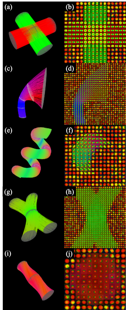
Fig. 3: Examples of artificial crossing (a,b), fanning (c,d), highly curved (e,f), kissing (g,h) and twisting (i,j) fibers as well as of the corresponding tensor images generated with Fiberfox.

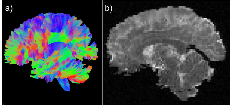
Fig. 4: Realistic simulation of a whole brain dataset with multiple artifacts.

Known Issues

If a scaling factor is applied to the selcted fiber bundle, the corresponding fiducials are not scaled accordingly.
In some cases the automatic update of the selected fiber bundle is not triggered even if "Real Time Fibers" is checked, e.g. if a fiducial is deleted. If this happens on can always force an update by pressing the "Generate Fibers" button.

If any other issues or feature requests arises during the use of Fiberfox, please don't hesitate to send us an e-mail or directly report the issue in our bugtracker: http://bugs.mitk.org/

References

[1] Neher, P.F., Laun, F.B., Stieltjes, B., Maier-Hein, K.H., 2014. Fiberfox: facilitating the creation of realistic white matter software phantoms. Magn Reson Med 72, 1460–1470. doi:10.1002/mrm.25045

[2] Neher, P.F., Laun, F.Neher, P.F., Stieltjes, B., Laun, F.B., Meinzer, H.-P., Fritzsche, K.H., 2013. Fiberfox: A novel tool to generate software phantoms of complex fiber geometries, in: Proceedings of International Society of Magnetic Resonance in Medicine.

[3] Neher, P.F., Stieltjes, B., Laun, F.B., Meinzer, H.-P., Fritzsche, K.H., 2013. Fiberfox: A novel tool to generate software phantoms of complex fiber geometries, in: Proceedings of International Society of Magnetic Resonance in Medicine.

[4] Hering, J., Neher, P.F., Meinzer, H.-P., Maier-Hein, K.H., 2014. Construction of ground-truth data for head motion correction in diffusion MRI, in: Proceedings of International Society of Magnetic Resonance in Medicine.