Table of Contents
Introduction
This views offers a generic fitting component for time resolved image data.
Contact information
If you have any questions, need support, find a bug or have a feature request, feel free to contact us at www.mitk.org.
Citation information
If you use the view for your research please cite our work as reference:
Debus C and Floca R, Ingrisch M, Kompan I, Maier-Hein K, Abdollahi A, Nolden M, MITK-ModelFit: generic open-source framework for model fits and their exploration in medical imaging – design, implementation and application on the example of DCE-MRI. https://doi.org/10.1186/s12859-018-2588-1 (BMC Bioinformatics 2019 20:31)
Time series and mask selection
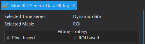
In principle, every model can be fitted on the entire image. However, for model configuration reasons and computational time cost, this is often not advisable. Therefore, apart from the image to be fitted (Selected Time Series), a ROI segmentation can be defined (Selected Mask), within which model fitting is performed. The view currently offers Pixel based and/or ROI based averaged fits of time-varying curves. The ROI based fitting option becomes enabled, if a mask is selected.
Supported models
Currently the following models are available for fitting:
- Linear model : y = offset + slope*x
- Generic parameter model : A simple formula can be manually provided and will be parsed for fitting.
- T2 decay model : y = A*exp(-t/B)
Model settings
Model specific settings
Selecting one of the supported models will open below tabs for further configuration of the model.
- The Generic parameter model required as input a formula to be parsed and the number parameters to fit. In the following image, detailed formula information is given.
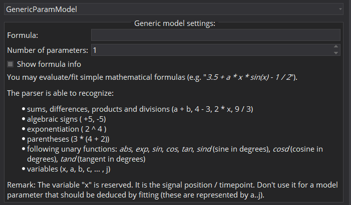 Formula info for the generic parameter model
Start parameter
In cases of noisy data it can be useful to define the initial starting values of the parameter estimates, at which optimization starts, in order to prevent optimization results in local optima. Each model has default scalar values (applied to every voxel) for initial values of each parameter, however these can be adjusted. Moreover, initial values can also be defined locally for each individual voxel via starting value images. To load a starting value image, change the Type from scalar to image. This can be done by double-clicking on the type cell. In the Value column, selection of a starting value image will be available.
Constraints settings
To limit the fitting search space and to exclude unphysical/illogical results for model parameter estimates, constraints to individual parameters as well as combinations can be imposed. Each model has default constraints, however, new ones can be defined or removed by the + and – buttons in the table. The first column specifies the parameter(s) involved in the constraint (if multiple parameters are selected, their sum will be used) by selection in the drop down menu. The second column Type defines whether the constraint defines an upper or lower boundary. Value defines the actual constraint value, that should not be crossed, and Width allows for a certain tolerance width.
Executing a fit
In order to distinguish results from different model fits to the data, a Fitting name can be defined. As default, the name of the model and the fitting strategy (pixel/ROI) are given. This name will then be appended by the respective parameter name.
For development purposes and evaluation of the fits, the option Generate debug parameter images is available. Enabling this option will result in additional parameter maps displaying the status of the optimizer at fit termination. In the following definitions, an evaluation describes the process of cost function calculation and evaluation by the optimizer for a given parameter set.
- Stop condition: Reasons for the fit termination, i.e. criterion reached, maximum number of iterations,...
- Optimization time: The overall time from fitting start to termination.
- Number of iterations: The number of iterations from fitting start to termination.
After all necessary configurations are set, the button Start Modelling is enabled, which starts the fitting routine. Progress can be seen in the message box on the bottom. Resulting parameter maps will afterwards be added to the Data Manager as sub-nodes of the analyzed 4D image.