|
Medical Imaging Interaction Toolkit
2016.11.0
Medical Imaging Interaction Toolkit
|
|
Medical Imaging Interaction Toolkit
2016.11.0
Medical Imaging Interaction Toolkit
|

Available sections:
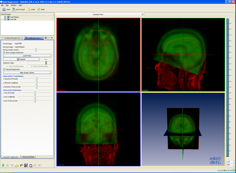
This view allows you to register 2D as well as 3D images in a rigid manner. If the Moving Image is an image with multiple timesteps you can select one timestep for registration. Register means to align two images, so that they become as similar as possible. Therefore you can select from different transforms, metrics and optimizers. Registration results will directly be applied to the Moving Image. Also binary images as image masks can be used to restrict the metric evaluation only to the masked area.
This document will tell you how to use this view, but it is assumed that you already know how to navigate through the slices of an image using the multi-widget.
Depending on your system the registration can fail to allocate memory for calculating the gradient image for registration. In this case you can try to select another optimizer which is not based on a gradient image and uncheck the checkbox for "Compute Gradient".
First of all you have to open the data sets which you want to register and select them in the Data Manager. You have to select exactly 2 images for registration. The image which was selected first will become the fixed image, the other one the moving image. The two selected images will remain for registration until exactly two images were selected in the Data Manager again.
While there aren't two images for registration a message is viewed on top of the view saying that registration needs two images. If two images are selected the message disappears and the interaction areas for the fixed and moving data appears. If both selected images have a binary image as childnode a selection box appears which allows, when checked, to use the binary images as image mask to restrict the registration on this certain area. If an image has more than one binary image as child, the upper one from the DataManager list is used. If the Moving Image is a dynamic images with several timesteps a slider appears to select a specific timestep for registration.
On default only the fixed and moving image are shown in the render windows. If you want to have other images visible you have to set the visibility via the Data Manager. Also if you want to perform a reinit on a specific node or a global reinit for all nodes you have to use the Data Manager.
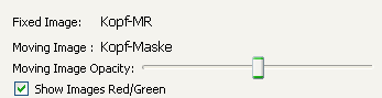
The colour of the images can be changed between grey values and red/green and the opacity of the moving image can be changed. With the "Moving Image Opacity:" slider you can change the opacity of the moving dataset. In the "Show Images Red/Green" you can switch the color from both datasets. If you check the box, the fixed dataset will be displayed in red-values and the moving dataset in green-values to improve visibility of differences in the datasets. If you uncheck the "Show Images Red/Green" checkbox, both datasets will be displayed in grey-values.
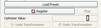
In the "Register" area you can start the registration by clicking the "Calculate Transform" button. The optimizer value for every iteration step is diplayed as LCD number next to the "Optimizer Value:" label. Many of the registration methods can be canceled during their iteration steps by clicking the "Stop Optimization" button. During the calculation, a progress bar indicates the progress of the registration process. The render widgets are updated for every single iteration step, so that the user has the chance to supervise how good the registration process works with the selected methods and parameters. If the registration process does not lead to a sufficient result, it is possible to undo the transformation and restart the registration process with some changes in parameters. The differences in transformation due to the changed parameters can be seen in every iteration step and help the user understand the parameters. Also the optimizer value is updated for every single iteration step and shown in the GUI. The optimizer value is an indicator for the misalignment between the two images. The real time visualization of the registration as well as the optimizer value provides the user with information to trace the improvement through the optimization process. The "Undo Transformation" button becomes enabled when you have performed an transformation and you can undo the performed transformations. The "Redo Transformation" button becomes enabled when you have performed an undo to redo the transformation without to recalculate it.
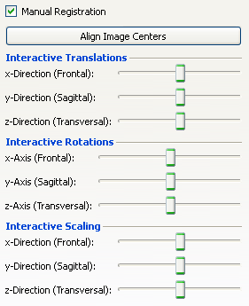
In the "Manual Registration" area, shown by checking the checkbox Manual Registration, you can manually allign the images by moving sliders for translation and scaling in x-, y- and z-axis as well as for rotation around the x-, y- and z-Axis. Additionally you can automatically allign the image centers with the button "Automatic Allign Image Centers".
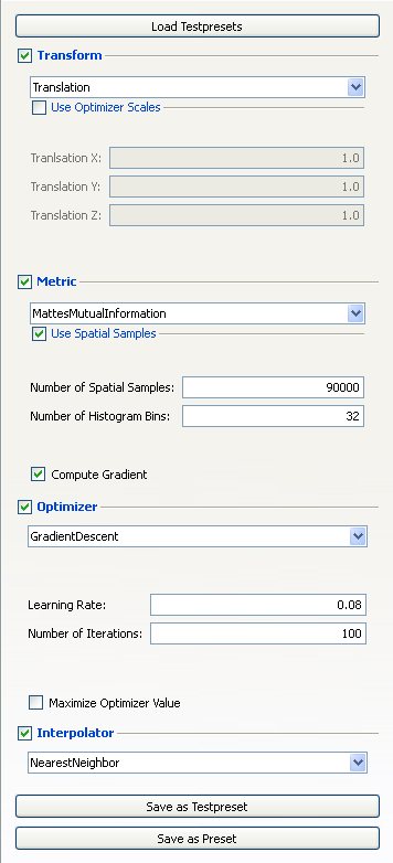
In the "Advanced Mode" tab you can choose a transform, a metric, an optimizer and an interpolator and you have to set the corresponding parameters to specify the registration method you want to perform. With the topmost button you can also load testpresets. These presets contain all parametersets which were saved using the "Save as Testpreset" button. The "Save as Preset" button makes the preset available from the "Automatic Registration" tab. This button should be used when a preset is not intended for finding good parameters anymore but can be used as standard preset.
To show the current transform and its parameters for the registration process, the Transform checkbox has to be checked. Currently, the following transforms are implemented (for detailed information see [1] and [2]):
The desired transform can be chosen from a combo box. All parameters defining the selected transform have to be specified within the line edits and checkboxes underneath the transform combo box. To show the current metric and its parameters for the registration process, the Metric checkbox has to be checked. Currently, the following metrics are implemented (for detailed information see [1] and [2]):
The desired metric can be chosen from a combo box. All parameters defining the selected metric have to be specified within the line edits and checkboxes underneath the metric combo box. To show the current optimizer and its parameters for the registration process, the Optimizer checkbox has to be checked. Currently, the following optimizers are implemented (for detailed information see [1] and [2]):
The desired optimizer can be chosen from a combo box. All parameters defining the selected optimizer have to be specified within the line edits and checkboxes underneath the optimizer combo box. To show the current interpolator for the registration process, just check the Interpolator checkbox. Currently, the following interpolators are implemented (for detailed information see [1] and [2]):
You can show and hide the parameters for the selection by checking or unchecking the corresponding area. You can save the current sets of parameters with the "Save as Testpreset" or "Save as Preset" buttons.
 1.8.9.1
